
Sooner or later, a column lands on your desk where every value has the useful bit buried in the middle. Think of a product code like PRD-2026-XL where you only want the year, or an account reference where the branch sits between two fixed markers. You do not want the start, you do not want the end, you want the piece in between. That is exactly the job the "Mid" function was built for.
The "Mid" function pulls a chunk of characters out of a text string, starting at a position you choose and grabbing as many characters as you ask for. If you work in Excel with imported data, reference codes, or anything with a predictable layout, this is one of those small functions you will reach for again and again.
Where to find it?
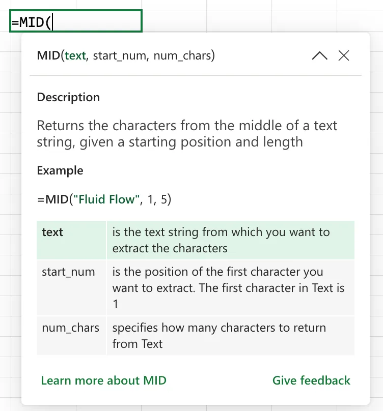
You type the "Mid" function straight into a cell. Start with an equals sign, type MID, and Excel's formula AutoComplete will offer it and show you the three arguments it expects. You can also reach it through the Formulas tab, "Insert Function", and the Text category if you prefer the guided dialog. It behaves the same in Excel for Windows, Excel for Mac, and Excel for the web.
The "Left" function takes characters from the start of the text and the "Right" function takes them from the end. The "Mid" function is the only one of the three that starts at an arbitrary position, which is why it needs both a start position and a length. If you only ever need the beginning or the end, the "Left" or "Right" function is simpler.
Usage
The "Mid" function takes three arguments, and all three are required. You give it the text to look inside, the position where it should start, and how many characters to grab from there.
=MID(text, start_num, num_chars)
| Parameter | Required | Type | Description |
|---|---|---|---|
| text | Yes | Text | The text string that contains the characters you want to extract |
| start_num | Yes | Number | The position of the first character to extract. The first character in the text is position 1 |
| num_chars | Yes | Number | How many characters to return, starting from start_num |
The key thing to hold on to is that the "Mid" function counts positions starting at 1, not 0. The first character is position 1, the second is position 2, and so on. Let us walk through how it behaves with the values it can meet.
A straightforward extraction from the middle of a word looks like this.
Data in A1
"Manuel Gomes"

=MID(A1, 8, 5)

will return

"Gomes"
Position 8 is the "G" in "Gomes", and five characters get you the whole surname.
The "Mid" function always returns text, even when the characters it extracts are digits. This matters if you plan to do math with the result.
Data in A1
"PRD-2026-XL"

=MID(A1, 5, 4)

will return

"2026"
That 2026 is text, not a number. If you need it as a number for a calculation, wrap the result in the "Value" function or multiply it by 1.
Numbers passed as the text argument are converted to text first, then sliced. Excel does the conversion for you, so you do not get an error, but you are extracting from the digits of the number.
Data in A1
12345

=MID(A1, 2, 3)

will return

"234"
If you ask for more characters than remain, the "Mid" function simply stops at the end of the text rather than erroring or padding with spaces.
Data in A1
"Porto"

=MID(A1, 4, 50)

will return

"to"
There are only two characters from position 4 onward, so that is what you get back.
The function family
The "Mid" function belongs to the text-extraction family. These are the functions people reach for when they need to slice strings apart. None of them have a dedicated article yet, so keep this table handy.
| Function | What it does |
|---|---|
| Mid | Extracts characters from the middle, given a start and a length |
| Left | Extracts a number of characters from the start of the text |
| Right | Extracts a number of characters from the end of the text |
| Len | Returns how many characters are in the text |
| Find | Returns the position of one string inside another, case sensitive |
| Search | Returns the position of one string inside another, case insensitive |
| Textsplit | Splits text into multiple cells by a delimiter (Microsoft 365) |
The "Mid" function truly shines when you pair it with the "Find" or "Search" function, because those give you a start position to feed in when the useful part does not sit at a fixed spot.
Real-world examples
Pulling the year out of a reference code
Say column A holds codes like PRD-2026-XL, PRD-2025-SM, and so on, where the four-digit year always starts at position 5. Joana wants just the year in a helper column.
=MID(A2, 5, 4)
This returns 2026 as text. If she needs it as a real number for sorting or math, she wraps it: =VALUE(MID(A2, 5, 4)).
Extracting a value between two markers
When the piece you want does not sit at a fixed position, let the "Find" function locate it for you. Imagine a cell holding Name: Maria; City: Aveiro and you want just the name.
=MID(A2, FIND(":", A2) + 2, FIND(";", A2) - FIND(":", A2) - 2)
The first "Find" function locates the colon, and the + 2 steps past the colon and the space that follows it, so the extraction starts on the "M". The second "Find" function locates the semicolon, and the - 2 trims those same two characters back off the length. The result is Maria. It looks busy, but it is just the "Mid" function with calculated start and length arguments.
Grabbing a single character
Because num_chars can be 1, the "Mid" function is a clean way to read one character from a known position, such as a status flag in the middle of a code.
=MID(A2, 3, 1)
Non-intuitive behaviors
Positions are 1-based, not 0-based
If you come from a programming background, this catches you every time. The first character is position 1, so to start at the very beginning you pass 1, not 0. Passing 0 is not a valid start and will error.
Dates and times are extracted from their serial number
Excel stores dates and times as serial numbers, and the "Mid" function sees that underlying number, not the formatted date you read on screen. A cell showing 01/01/2026 is really a number under the hood, so slicing it with =MID(A1, 1, 2) returns the first digits of that serial number, not 01.
If you actually want to pull characters out of a formatted date, convert it to text first with the "Text" function, for example =MID(TEXT(A1, "dd/mm/yyyy"), 1, 2). Otherwise you are slicing the serial number and the result will look nothing like the date.
The result is always text
Even when every extracted character is a digit, the "Mid" function hands back text. It will still look right in the cell, but a later "Sum" function or a comparison against a number may behave unexpectedly. Wrap the result in the "Value" function, or multiply by 1, when you need a genuine number.
Limitations
All three arguments are required
Unlike some text functions, the "Mid" function will not assume a default. You must supply text, start_num, and num_chars, otherwise Excel rejects the formula. If you only want characters from one end, the "Left" or "Right" function is the better fit because it asks for one number instead of two.
It works on characters, not words or delimiters
The "Mid" function has no idea what a word, a space, or a separator is. It counts raw characters. To extract by a delimiter you have to compute the positions yourself with the "Find" or "Search" function, or move to the "Textsplit" function on Microsoft 365.
Invalid positions return an error or an empty string
A start_num below 1 returns #VALUE!, and a negative num_chars also returns #VALUE!. A start_num past the end of the text returns an empty string rather than an error, so a column can end up with blank cells and no warning. Check the text length with the "Len" function before you rely on a fixed start position.
Localization
The "Mid" function name is the same across regional settings, but the argument separator is not. With comma-based settings you separate the arguments with commas, and with semicolon-based settings, such as Portugal, you use semicolons.
// Comma-based regional settings
=MID(A1, 5, 4)

// Semicolon-based regional settings (for example, Portugal)
=MID(A1; 5; 4)
Troubleshooting Common Errors
The formula returns #VALUE!
Cause: The start_num is less than 1 or the num_chars is negative. This often happens when start_num is calculated with another formula, for example a "Find" function that failed to locate its target and returned an error, which then cascades into the "Mid" function.
Solution: Make sure start_num is at least 1 and num_chars is zero or greater. When you build the position with the "Find" function, guard it so a missing match does not push the position below 1.
=IFERROR(MID(A1, FIND("-", A1) + 1, 4), "")
The result is blank when the cell clearly has text
Cause: The start_num is larger than the length of the text, so there is nothing at that position to extract, and the "Mid" function returns an empty string.
Solution: Check the string length with the "Len" function and confirm your start position actually falls inside it. Recalculate start_num if it was derived from another cell.
The extracted number will not add up
Cause: The "Mid" function returns text, so a digit string like "2026" is not treated as the number 2026 in later math.
Solution: Convert the result to a number with the "Value" function or by multiplying by 1.
=VALUE(MID(A1, 5, 4))
Slicing a date gives strange numbers
Cause: The cell holds a real date, which Excel stores as a serial number, and the "Mid" function is reading that number rather than the formatted date.
Solution: Convert the date to text with the "Text" function before extracting.
=MID(TEXT(A1, "dd/mm/yyyy"), 4, 2)
Recommendations
Here are some things to keep in mind.
Let the "Find" function calculate the position
Hard-coding a start_num only works when the useful part always sits at the same spot. When it moves, compute the position with the "Find" or "Search" function so the formula adapts to each row instead of breaking on the first exception.
=MID(A1, FIND("-", A1) + 1, 4)
Convert to a number when you need one
Remember that the "Mid" function always returns text. If the extracted value feeds a calculation, a sort, or a lookup that expects a number, wrap it so it stops being text.
=VALUE(MID(A1, 5, 4))
Always deal with errors
A start position that drops below 1, or a "Find" function that fails to locate its marker, will surface as #VALUE! and can cascade into every formula that reads the result. Wrap the "Mid" function in the "Iferror" function so one awkward row does not break the report that depends on it.
=IFERROR(MID(A1, FIND("-", A1) + 1, 4), "")
Final Thoughts
The "Mid" function is a small, sharp tool for pulling a piece out of the middle of a string. Remember that it counts from position 1, that it always returns text, and that pairing it with the "Find" function is what turns it from a rigid formula into one that adapts to your data. Keep those three points in mind and it will handle almost any string-slicing job you throw at it.
Sources
Back to the Excel Function Reference
Photo by Ksenia Makagonova on Unsplash


No comments yet
Be the first to share your thoughts on this article!