
The "Sumif" function is a super important one and it filters information so that you only sum the values you actually need.
For example, you have a sheet of expenses. One column says what the expense was for, another says how much it cost, and someone wants to know how much went on food, travel, or hotels. Then with the "Sumif" function you can get a total for each category. Add a new row and the value is summed automatically.
The "Sumif" function adds up numbers, but only for the rows that meet a condition you set. If you already use the "Sum" function in Excel to total a column, think of this one as the same thing with a filter attached.
Where to find it?
You type the "Sumif" function directly into a cell. Start with an equals sign, type SUMIF, and Excel's formula AutoComplete shows you the signature as you fill in each argument. The Formulas tab and its "Insert Function" dialog give you the same thing with a guided form if you prefer. It behaves identically in Excel for Windows, Excel for Mac, and Excel for the web.
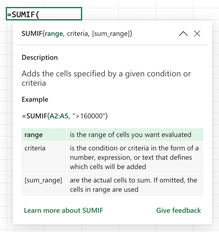
The argument order is reversed between the two. The "Sumifs" function puts the range to add first, =SUMIFS(sum_range, criteria_range, criteria). The "Sumif" function puts it last, =SUMIF(range, criteria, [sum_range]). Copying a formula from one to the other without swapping the arguments is the most common reason a total comes back wrong.
Usage
You give the "Sumif" function a range to test, the condition each cell in that range must meet, and optionally a second range holding the numbers to add.
=SUMIF(range, criteria, [sum_range])
| Parameter | Required | Type | Description |
|---|---|---|---|
| range | Yes | Range | The cells checked against the condition |
| criteria | Yes | Value or expression | The condition a cell must meet to be included |
| sum_range | No | Range | The cells to add. Defaults to range if omitted |
Testing and summing the same column
When you leave out sum_range, Excel adds the very cells it tested. This is how you total everything above a threshold.
Data in A1:A5
100, 250, 50, 400, 75

=SUMIF(A1:A5, ">100")

will return

650
Testing one column and summing another
Most of the time the condition lives in one column and the money lives in another. Pass both and the function lines them up row by row.
Column A (Category)   Column B (Amount)
Travel                100
Software              200
Travel                150

=SUMIF(A2:A4, "Travel", B2:B4)

will return

250
Comparison operators
Criteria are not limited to exact matches. Wrap the operator and the value together inside quotation marks. The available operators are >, <, >=, <=, and <> for "not equal to".
=SUMIF(B2:B100, "<>Travel", C2:C100)
Criteria that live in a cell
Hardcoding a threshold inside a formula means editing the formula every time it changes. Put the value in its own cell instead, then join the operator to that cell with the & symbol. The & symbol glues two pieces of text together, so ">"&E1 becomes ">100" when E1 holds 100.
=SUMIF(B2:B100, ">"&E1, C2:C100)
Wildcards for partial text
Text criteria accept two wildcard characters. A ? stands for any single character, and a * stands for any run of characters. This totals every category beginning with "Trav".
=SUMIF(A2:A100, "Trav*", B2:B100)
To match a literal ? or * in your data, put a tilde ~ in front of it.
What happens to each kind of value
Inside sum_range, numbers are added, blank cells contribute nothing, and text is skipped rather than causing a failure. Dates and times are stored internally as numbers, so they get added like any other number, which is rarely what you want. Error values are the exception: one #N/A or #DIV/0! in sum_range and the formula returns that error instead of a total.
The function family
The "Sumif" function sits in a group of conditional aggregates that are easy to mix up. Pick by how many conditions you have and what you want back.
| Function | What it does |
|---|---|
| Sum | Adds everything, no conditions |
| Sumif | Adds the values that meet one condition |
| Sumifs | Adds the values that meet several conditions |
| Countif | Counts the rows that meet one condition |
| Averageif | Averages the values that meet one condition |
Real-world examples
A category total that updates itself
Manuel tracks household expenses and wants one cell per category on a summary tab. With the category name sitting in E1, a single formula covers it and picks up every new row as he adds them.
=SUMIF(Category, E1, Amount)
Here Category and Amount are named ranges, which are labels you assign to a range so the formula reads like a sentence instead of a set of coordinates.
Everything from a date onwards
Because dates are numbers underneath, comparison operators work on them directly. This totals every amount recorded on or after the date in F1.
=SUMIF(D2:D500, ">="&F1, C2:C500)
Edge Cases
A mismatched sum_range gets silently reshaped
If sum_range is a different size from range, the "Sumif" function does not complain. It takes the top left cell of sum_range as a starting point and then adds a block the same size and shape as range. So =SUMIF(A2:A9, "Travel", C2:C18) quietly adds C2:C9 and ignores the rest.
That is convenient when the top left cell is right and a real problem when it is not, because the answer looks reasonable and nobody checks. Always give both ranges the same rows.
=SUMIF(A2:A100, "Travel", C5:C103) adds C5:C13 against categories from row 2, so every row is matched against the wrong amount. Line the ranges up on identical rows and the problem disappears.
Text criteria are not case sensitive
"Travel", "travel", and "TRAVEL" all match each other. If you need to tell them apart, the "Sumif" function cannot do it. Use the "Sumproduct" function combined with the "Exact" function instead, which compares text character by character including case.
Trailing spaces stop a match you can see with your own eyes
A cell that reads Travel with a space on the end never matches "Travel", and nothing on screen tells you why. Clean the column with the "Trim" function, which removes leading and trailing spaces, and the total appears.
Limitations
Only one condition
The "Sumif" function tests exactly one condition. The moment you need two, such as travel expenses in a given month, move to the "Sumifs" function rather than trying to nest anything.
Criteria longer than 255 characters break
Microsoft documents that the function returns incorrect results when matching strings longer than 255 characters. Compare against a shortened value using the "Left" function, or match on an identifier column instead of the long text.
An error in sum_range takes over the result
A single #N/A, #DIV/0!, or #VALUE! inside sum_range makes the whole formula return that error. It does not skip the bad cell the way it skips text. Fix the source cell, or wrap the formula in the "Iferror" function so a report does not go blank because of one row.
Localization
The character separating arguments depends on your regional and list separator settings. Some settings use a comma, others, such as Portugal, use a semicolon.
// Comma-based regional settings
=SUMIF(A2:A100, "Travel", B2:B100)

// Semicolon-based regional settings (for example, Portugal)
=SUMIF(A2:A100; "Travel"; B2:B100)
Troubleshooting Common Errors
The formula returns 0
Cause: Either nothing matches the criteria, or the values in sum_range are numbers stored as text. Excel does not add text, so "45" stored as text contributes nothing. A small green triangle in the corner of a cell is the usual giveaway.
Solution: Test the match first with the "Countif" function to see whether any row qualifies. If rows do qualify but the total stays at 0, convert the column with Data, then Text to Columns, then Finish.
=COUNTIF(A2:A100, "Travel")
An operator in the criteria is ignored
Cause: The operator was left outside the quotation marks, or a cell reference was placed inside them. Excel then reads the whole thing as a literal value to match rather than a comparison.
Solution: Keep the operator inside the quotes and join any cell reference with &.
=SUMIF(B2:B100, ">="&E1, C2:C100)
The total is wrong but no error appears
Cause: range and sum_range cover different rows, so the function reshaped sum_range and matched the wrong amounts against your categories.
Solution: Check that both ranges start and end on the same rows. Named ranges or a formatted table make this automatic.
Recommendations
Give both ranges identical rows
Since a mismatch is corrected silently rather than flagged, the safest habit is to decide your row span once and reuse it for both arguments. Named ranges do this for you and keep the formula readable months later.
Keep the criteria in a cell
Put the category name or threshold in its own cell and point the formula at it. You change one cell instead of editing a formula, and a colleague opening the workbook can see what is being filtered without reading the formula bar.
=SUMIF(A2:A100, E1, B2:B100)
Move up to the "Sumifs" function early
If there is any chance a second condition will appear, write the "Sumifs" function from the start. It handles one condition perfectly well, and you avoid rewriting the formula (and reversing the argument order) later.
Always deal with errors
One error value in sum_range replaces your total with that error. Wrap the formula in the "Iferror" function or clean the source data so a single bad cell does not break the report that depends on it.
=IFERROR(SUMIF(A2:A100, "Travel", B2:B100), 0)
Final Thoughts
The "Sumif" function turns a filter-and-total chore into one formula that keeps working as rows pile up. Remember that the range to add comes last, that both ranges need to cover the same rows, and that a second condition means reaching for the "Sumifs" function. Those three things cover almost everything that goes wrong with it.
Sources
Back to the Excel Function Reference
Photo by Flow Clark on Unsplash


No comments yet
Be the first to share your thoughts on this article!