
Sooner or later every spreadsheet hands you a value where only the tail end matters. A product code where the last three characters are the warehouse, an invoice number where the final digits are the year, a phone number where you only care about the last four. This is the moment the "Right" function was built for.
The "Right" function reaches into a piece of text and pulls out a chosen number of characters counting from the end. If you work in Excel often, it quickly becomes one of those small tools you reach for without thinking, usually alongside its mirror image, the "Left" function, and its more flexible cousin, the "Mid" function. It looks almost too simple to need a reference, and then a stray trailing space or a currency value returns something unexpected, which is exactly why it earns one.
Where to find it?
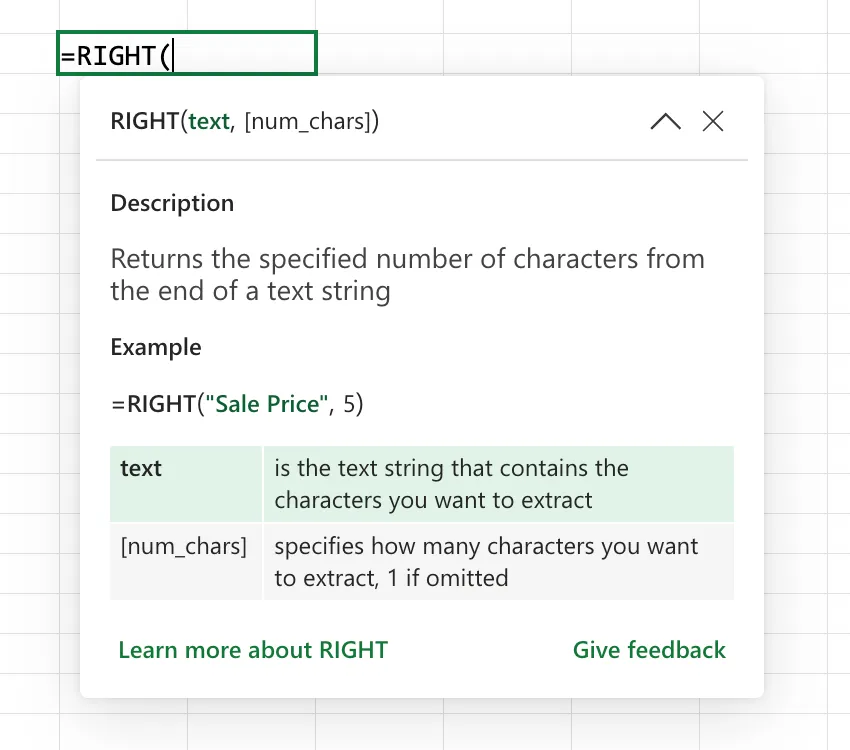
You type the "Right" function straight into a cell. Start with an equals sign, type RIGHT, and Excel will offer it through formula AutoComplete along with the argument tooltip. You can also reach it through the Formulas tab, then "Text", then "Insert Function", if you prefer the guided dialog. It behaves the same in Excel for Windows, Excel for Mac, and Excel for the web, and it has been part of Excel for so long that the version does not matter.
The "Right" function counts from the end of the text, while the "Left" function counts from the start. They take the same arguments and feel identical, so it is easy to grab the wrong one and wonder why your result is coming from the wrong side of the string. If you need characters from somewhere in the middle, neither one fits, and you want the "Mid" function instead.
Usage
The syntax is short. You give the "Right" function a piece of text and, optionally, how many characters you want from the end of it.
=RIGHT(text, [num_chars])
| Parameter | Required | Type | Description |
|---|---|---|---|
| text | Yes | Text | The text string you want to extract characters from |
| num_chars | No | Number | How many characters to take from the end. Defaults to 1 |
The interesting part is how the "Right" function reacts to the different kinds of values you can feed it, because it always thinks in terms of text even when the cell does not look like text. Let's take a look.
Ordinary text is the easy case. The "Right" function counts characters from the end and hands them back.
Data in A1
"Manuel Gomes"

=RIGHT(A1, 5)

will return

"Gomes"
If you leave out the second argument, the "Right" function assumes you want a single character.
Data in A1
"Porto"

=RIGHT(A1)

will return

"o"
Numbers are where people get surprised. The "Right" function does not see the number the way the cell displays it. It sees the underlying stored value and turns that into text first. So a cell that shows a tidy currency amount is, to the "Right" function, just the raw number with no symbol, no thousands separator, and no fixed decimals.
Data in A1 (cell displays $1,234.50)
1234.5

=RIGHT(A1, 2)

will return

".5"
Dates and times are numbers in disguise, since Excel stores them internally as serial numbers. The "Right" function reaches for that serial number, not the pretty date you see on screen, which is almost never what you want.
Data in A1 (cell displays 15/06/2026)
46188

=RIGHT(A1, 4)

will return

"6188"
Logical values are converted to their text form, so TRUE becomes the word "TRUE" and FALSE becomes "FALSE" before the extraction happens.
=RIGHT(TRUE, 1)

will return

"E"
A blank cell has nothing to extract, so the "Right" function politely returns an empty string.
Data in A1
(blank)

=RIGHT(A1, 3)

will return

""
Error values are not something the "Right" function can clean up. If the cell you point at holds an error, that same error comes straight back out.
Data in A1
#N/A

=RIGHT(A1, 2)

will return

#N/A
The function family
The "Right" function belongs to a small group of text functions that you end up using together, often nested inside one another. Keep this table handy for picking the right tool.
| Function | What it does |
|---|---|
| Right | Returns a number of characters from the end of the text |
| Left | Returns a number of characters from the start of the text |
| Mid | Returns characters from any position in the middle of the text |
| Len | Returns how many characters the text contains |
| Find | Returns the position of one string inside another, case sensitive |
The pairing that does the heavy lifting is the "Right" and "Len" functions together, or the "Right" and "Find" functions together, because they let you extract from the end without knowing the exact length in advance. Let's see an example of that below.
Real-world examples
Pulling a year suffix off an invoice number
João keeps invoice numbers in the shape INV-004821-26, where the last two digits are the year. He wants a plain year column for a pivot table.
=RIGHT(A2, 2)

will return

"26"
If he needs it as a real number rather than text, he wraps the result in the "Value" function so it can be totaled or sorted numerically.
Grabbing the last few digits of a phone number
Maria has a column of phone numbers and only wants the final four digits to match against another list.
=RIGHT(A2, 4)
This works cleanly as long as the numbers are stored as text. If they are stored as actual numbers, remember the "Right" function reads the raw value, so any formatting you applied is ignored.
Extracting a variable-length ending
When the tail you want is not a fixed length, you combine the "Right" function with the "Len" and "Find" functions to measure where to cut. Here Joana pulls the domain out of an email address by counting everything after the "@" sign.
=RIGHT(A2, LEN(A2) - FIND("@", A2))

will return

"manueltgomes.com"
The "Len" function gives the total length, the "Find" function locates the "@", and the subtraction tells the "Right" function exactly how many characters to keep.
Non-intuitive behaviors
Formatting is invisible to the function
The single biggest surprise is that the "Right" function ignores cell formatting entirely. A number formatted as currency, a percentage, or a date all get reduced to their stored value first. The $, the %, the thousands separators, and the calendar date you see are display only, and the "Right" function never sees them. If you truly need the last characters of the formatted string, convert the value to text with the "Text" function first, then apply the "Right" function to that.
num_chars of zero returns nothing
Passing zero as the second argument is valid and returns an empty string rather than an error. This is handy inside conditional formulas. If a calculated num_chars might land on zero and you always need at least one character back, guard it with the "Max" function, for example MAX(1, LEN(A2) - 5).
Asking for more than there is
If num_chars is larger than the length of the text, the "Right" function does not complain or pad the result. It simply returns the whole string, which makes it safe to over-ask when you are unsure of the length.
=RIGHT("Porto", 20)

will return

"Porto"
Limitations
It always returns text
Whatever goes in, a text string comes out, even when the source was a number. If the extracted characters need to behave as a number afterwards, you have to convert them back with the "Value" function or by multiplying by one. Forgetting this is the classic reason a later "Sum" or lookup against the result quietly fails.
A negative num_chars is an error
The second argument must be zero or greater. Anything below zero produces a #VALUE! error, so a calculation that feeds num_chars needs to be guarded against going negative.
It counts characters, not visible glyphs
The "Right" function counts every character stored in the cell, including trailing spaces and non-printing characters you cannot see. If the tail of your text is padding rather than real content, the function faithfully returns that padding, which is where most unexpected results come from. Clean the text with the "Trim" function first, as shown in the troubleshooting section below.
Emoji can count as two characters
Some symbols, such as emoji, are stored as a surrogate pair. That is two hidden code units that together make one visible character. Older versions of Excel count a surrogate pair as two characters, so asking for the last character of such a string can hand you back half a symbol.
To fix this, switch the workbook to Compatibility Version 2, which counts a surrogate pair as a single character. You set it under Formulas, then "Calculation Options", then "Compatibility Version". New workbooks in the Current Channel default to Version 2 as of April 2026.
Microsoft also marks the RIGHTB function as deprecated. RIGHTB is a variant that counts bytes instead of characters, used with double-byte languages such as Japanese, so use the "Right" function instead.
Localization
Excel translates function names in localized installs, so the "Right" function is not always called RIGHT on screen. In Portuguese it appears as DIREITA, and in French as DROITE. What saves you is that the formula stored in the file is always language neutral, written in English inside the workbook, and Excel translates it back to the display language when the file is opened. Share a workbook with a colleague running a different language version and the formula still works. It simply shows up under a different name.
The argument separator also changes with your regional and list separator settings. With some settings it is a comma, with others, such as Portugal, it is a semicolon.
// Comma-based regional settings, English display
=RIGHT(A2, 4)

// Semicolon-based regional settings, Portuguese display
=DIREITA(A2; 4)
Troubleshooting Common Errors
The result has an extra space or looks off by one character
Cause: The source text has one or more trailing spaces, or a non-breaking space (character code 160) that arrived with imported or web-copied data. The "Right" function counts those invisible characters just like any other.
Solution: Clean the text before extracting. The "Trim" function removes ordinary trailing spaces, and a "Substitute" function handles the stubborn non-breaking space.
=RIGHT(TRIM(SUBSTITUTE(A2, CHAR(160), " ")), 4)
The formula returns #VALUE!
Cause: The num_chars argument evaluated to a negative number, usually because it came from another calculation that went below zero.
Solution: Guard the argument so it never drops under zero, for example with the "Max" function, or check the inputs feeding it.
=RIGHT(A2, MAX(0, LEN(A2) - 5))
The result cannot be summed or matched as a number
Cause: The "Right" function always returns text, so digits it extracts are stored as text and will not behave numerically.
Solution: Wrap the result in the "Value" function to convert it back to a real number.
=VALUE(RIGHT(A2, 4))
The extracted characters are not what the cell shows
Cause: The source cell holds a number, date, or currency value, so the "Right" function is reading the raw stored value rather than the formatted display.
Solution: Convert the value to text in the format you actually see, using the "Text" function, then apply the "Right" function.
=RIGHT(TEXT(A2, "dd/mm/yyyy"), 4)
Recommendations
Let's look at some things to keep in mind.
Clean the text before you cut it
Trailing spaces and non-breaking characters are behind most surprising results. Wrapping the source in the "Trim" function, and dealing with character 160 when your data came from the web, saves a lot of confused debugging later.
Measure with Len and Find instead of hardcoding
When the ending you want is not a fixed length, resist typing a magic number. Combining the "Right" function with the "Len" and "Find" functions makes the formula adapt to each row automatically, so a longer or shorter value does not break it.
Convert numbers on purpose, in both directions
Because the "Right" function reads stored values and returns text, be deliberate at both ends. Use the "Text" function first when you care about the formatted look, and the "Value" function afterwards when you need a number back.
Always deal with errors
A single error value in the source cell passes straight through the "Right" function and into anything downstream. Wrap the formula in the "Iferror" function so one bad cell does not break the report that depends on it.
=IFERROR(RIGHT(A2, 4), "")
Final Thoughts
The "Right" function is one of those tools that feels trivial until a currency value or a trailing space returns something you did not expect. Remember that it always works on the stored value and always hands you text back, lean on the "Len" and "Find" functions when the length varies, and clean your input first. Keep those habits and it will quietly do its job in every report you build.
Sources
- RIGHT function on Microsoft Support
- Compatibility Versions on Microsoft Support
- Overview of formulas in Excel
Back to the Excel Function Reference
Photo by Andrea De Santis on Unsplash


No comments yet
Be the first to share your thoughts on this article!