
Picture a sales sheet that just keeps growing. One column holds the region, another holds the salesperson, another holds the amount, and your manager wants the total for the North region, but only for deals closed by Manuel, and only above a certain value. You could filter the table by hand every time, or you could write one formula that answers the question and keeps answering it as new rows arrive.
That is exactly what the "Sumifs" function does. It adds up the numbers in one range, but only for the rows that satisfy every condition you hand it. If you have used the "Sum" function in Excel to total a whole column, think of the "Sumifs" function as the same idea with a set of filters attached, so you total only the rows that matter.
Where to find it?
You type the "Sumifs" function straight into a cell. Start with an equals sign, type SUMIFS, and Excel's formula AutoComplete shows the signature as you fill in each argument. You can also reach it through the Formulas tab and the "Insert Function" dialog if you prefer a guided experience. It works the same way in Excel for Windows, Excel for Mac, and Excel for the web.
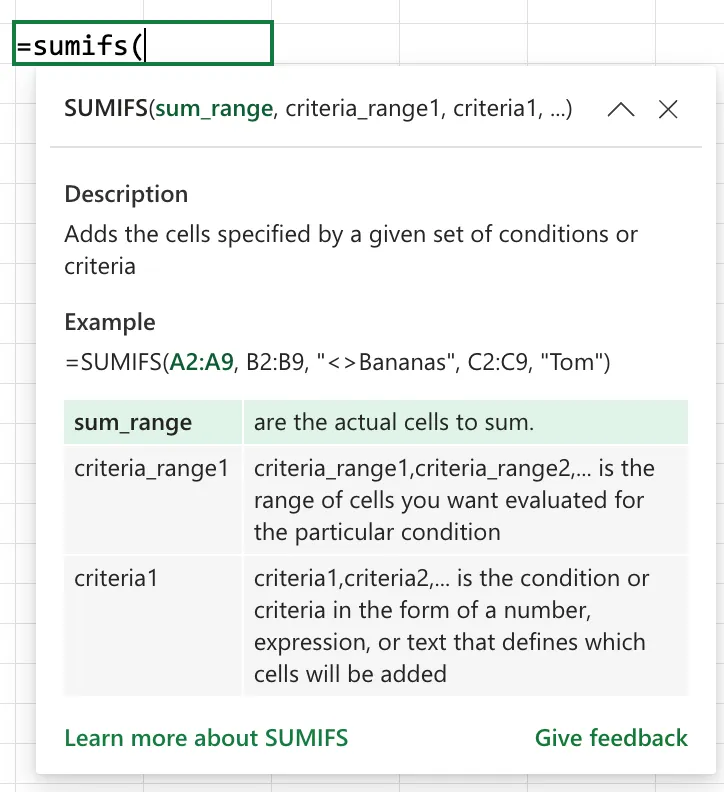
The "Sumif" function handles a single condition and puts the range to sum last: =SUMIF(range, criteria, [sum_range]). The "Sumifs" function handles several conditions and puts the range to sum first: =SUMIFS(sum_range, criteria_range1, criteria1, ...). That reversed argument order is the single most common reason a copied formula returns the wrong total, so check it whenever you switch between the two.
Usage
You give the "Sumifs" function the range you want to add, then one or more pairs of a criteria range and the criteria it must meet. Only the rows where every condition is true get added.
=SUMIFS(sum_range, criteria_range1, criteria1, [criteria_range2, criteria2], ...)
| Parameter | Required | Type | Description |
|---|---|---|---|
| sum_range | Yes | Range | The cells to add together |
| criteria_range1 | Yes | Range | The range tested against the first condition |
| criteria1 | Yes | Value or expression | The condition applied to criteria_range1 |
| criteria_range2, criteria2 | No | Range and condition | Additional pairs, up to 127 of them |
A single condition
At its simplest, the "Sumifs" function behaves like a filtered "Sum" function. Add up the amounts, but only for the North region.
Column A (Region)   Column B (Amount)
North               100
South               200
North               150

=SUMIFS(B2:B4, A2:A4, "North")

will return

250
Several conditions at once
Add a second pair and the conditions combine with AND logic. A row is included only when it satisfies all of them. Here we total the North region, but only the rows owned by Manuel.
Column A (Region)   Column B (Owner)   Column C (Amount)
North               Manuel             100
North               Maria              200
North               Manuel             150

=SUMIFS(C2:C4, A2:A4, "North", B2:B4, "Manuel")

will return

250
Comparison operators and cell references
Criteria are not limited to exact matches. Wrap an operator and a value in quotation marks to compare, and join an operator to a cell reference with the & symbol when the threshold lives in another cell.
=SUMIFS(C2:C100, C2:C100, ">500")

=SUMIFS(C2:C100, C2:C100, ">"&E1)
Wildcards for partial text
Text criteria accept ? to match any single character and * to match any run of characters. This totals every owner whose name starts with "Man".
=SUMIFS(C2:C100, B2:B100, "Man*")
The values inside sum_range follow the usual rules. Numbers are added, blank cells contribute nothing, and text is ignored. An error value sitting in sum_range is the exception: it does not get skipped, it takes over the whole result and the formula returns that error.
The function family
The "Sumifs" function sits in a small group of conditional aggregates that readers often mix up. None of these have a dedicated article yet, so keep this table handy while you pick the right one.
| Function | What it does |
|---|---|
| Sum | Adds everything you give it, with no conditions |
| Sumif | Adds the values that meet one condition |
| Sumifs | Adds the values that meet several conditions |
| Countifs | Counts the rows that meet several conditions |
| Averageifs | Averages the values that meet several conditions |
Real-world examples
A dashboard total that filters itself
Manuel keeps a running sheet of deals and wants a single cell that shows this quarter's revenue for one product. With the product name in E1 and the quarter start date in E2, one formula does the whole job and updates as new rows land.
=SUMIFS(Amount, Product, E1, CloseDate, ">="&E2)
Summing between two dates
Two date conditions on the same range give you a window. This totals the amounts closed during a single month.
=SUMIFS(C2:C500, D2:D500, ">="&F1, D2:D500, "<="&F2)
Here F1 holds the first day of the month and F2 holds the last, so every deal inside that range gets counted and nothing outside it does.
Edge Cases
The ranges must be the same shape
Every criteria_range has to have the same number of rows and columns as sum_range. If they differ, the "Sumifs" function returns a #VALUE! error rather than a partial answer. This bites most often when one range is B2:B100 and another is C2:C101, an off-by-one slip that is easy to miss.
=SUMIFS(C2:C100, A2:A100, "North", B2:B99, "Manuel") fails because the last range stops one row short. Keep every range on the same rows.
Text criteria ignore trailing spaces you cannot see
If a criterion looks correct but the total comes back as 0, the culprit is often invisible spaces in the source data, usually left behind by a copy from a web page or another system. The value in the cell reads "Manuel " with a trailing space, so it never matches "Manuel". Cleaning the column with the "Trim" function fixes it.
Dates are compared by value, not by appearance
A cell can display "Jul-16" while actually holding a full date serial number underneath. The "Sumifs" function compares the underlying value, not the formatted text, so build date criteria from real dates (or a cell that holds one) rather than the string you see on screen.
Limitations
Conditions are always AND, never OR
Every criteria pair you add narrows the result further, because they combine with AND logic. There is no built-in way to say "region is North OR South" inside a single "Sumifs" function. For an OR across conditions, add two "Sumifs" functions together or move to the "Sumproduct" function.
=SUMIFS(C2:C100, A2:A100, "North") + SUMIFS(C2:C100, A2:A100, "South")
A maximum of 127 criteria pairs
You can supply up to 127 range and criteria pairs to a single "Sumifs" function. In real workbooks you rarely pass more than two or three, so this ceiling almost never matters, but it exists.
An error in the sum range stops the total
If any cell in sum_range holds an error value such as #N/A, #DIV/0!, or #VALUE!, the "Sumifs" function returns that same error instead of a number. It does not step around the bad cell the way it ignores text, so a single poisoned value can take down an otherwise correct report.
Localization
The separator between arguments changes with your regional and list separator settings. With some settings it is a comma, with others, such as Portugal, it is a semicolon.
// Comma-based regional settings
=SUMIFS(C2:C100, A2:A100, "North", B2:B100, "Manuel")

// Semicolon-based regional settings (for example, Portugal)
=SUMIFS(C2:C100; A2:A100; "North"; B2:B100; "Manuel")
Troubleshooting Common Errors
The formula returns 0 when you expected a total
Cause: No row satisfies every condition at once, or the criteria do not match the data. Common reasons are trailing spaces in the source text, numbers stored as text in the sum range, or a date criterion written as a string instead of a real date.
Solution: Loosen the formula to one condition at a time to see which one filters everything out, and clean the offending column. The "Trim" function removes stray spaces, and the "Value" function converts text that should be a number.
=SUMIFS(C2:C100, B2:B100, TRIM(E1))
The formula returns #VALUE!
Cause: One of the ranges is a different size from sum_range. The "Sumifs" function requires every range to cover the same rows and columns.
Solution: Check that each criteria_range starts and ends on the same rows as sum_range. Fixing an off-by-one range usually clears the error immediately.
Criteria with an operator are not filtering
Cause: The operator and value were not written as text, or a cell reference was joined without the & symbol, so Excel reads the whole thing as a plain value.
Solution: Put the operator inside quotation marks and concatenate any cell reference with &.
=SUMIFS(C2:C100, C2:C100, ">"&E1)
Recommendations
Here are some things to keep in mind.
Point every range at the same rows
Because all ranges must share the same shape, decide on your row span once and reuse it for every argument. Named ranges make this almost automatic and keep a long formula readable.
=SUMIFS(Amount, Region, "North", Owner, "Manuel")
Keep thresholds in cells, not inside the formula
When a condition is a moving target, such as a cut-off amount or a start date, put it in its own cell and reference it with &. You change one cell instead of editing the formula, and the intent stays obvious to whoever opens the workbook next.
=SUMIFS(C2:C100, C2:C100, ">="&E1)
Always deal with errors
A single error value in the sum range takes over the whole result, so it is worth catching before it reaches a dashboard or a report a colleague depends on. Wrap the formula in the "Iferror" function or clean the source data so one bad cell does not erase an otherwise correct total.
=IFERROR(SUMIFS(C2:C100, A2:A100, "North"), 0)
Final Thoughts
The "Sumifs" function turns a filter-and-total chore into a single formula that keeps working as your data grows. Remember that the range to sum comes first, that every range has to line up on the same rows, and that all your conditions combine with AND rather than OR. Get those three right and it becomes one of the most dependable tools in your workbook.
Sources
Back to the Excel Function Reference
Photo by Nick Fewings on Unsplash



No comments yet
Be the first to share your thoughts on this article!