
Everyone uses Excel in one way or another, so the next logical step is to integrate it with Power Automate and create some automation on your data, either by adding or removing rows, doing reports, or doing data synchronization (if you value your sanity, don’t do data synchronization, trust me).
Power Automate has many Excel actions, but some of them require an ID to work. Excel doesn’t have an ID column, so if we want to get the data, we would need to create one.
There are many ways to do this, and I’ve seen a few, but let’s look at the one that works better in my experience.
The "problem": Where’s the Excel ID?
We can see this "problem" when we try to do execute a “Update Row” action for example.
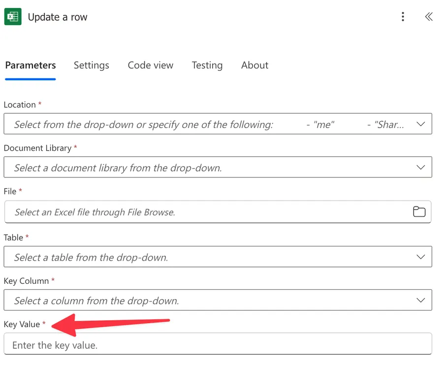
We see a “Key Column” and “Key Value,” but we don’t have one. Excel doesn’t automatically generate a key column that we can use. It has a function called “Row(),” but this will change each time we add a new row. If we want the ID to identify the row, then we can’t have it changed; otherwise, we would be updating different values, if the user inserts data in the middle of the table, for example.
I’ve also seen some plugins that do this, but let’s try to use what we have.
Here’s what we want to achieve
If we want the system to work, let's define the requirements or at least the things that we would like it to do.
- We want the Excel ID to be created once and not change over time. This way we are sure that we can reference the same ID and it always points to the correct value (unless the use changes it or is deleted)
- We want unique IDs so that, regardless of the document size, we’re always sure that the value is unique.
- We don’t want an Excel ID for empty rows. A table can have empty rows, and we don’t want to pull them to Power Automate each time we do a “List rows present in a table Action,” for example.
- We want to trigger it from Power Automate to automate the process.
- We want the same solution even if multiple Excel ID columns are in the same table. The person may have one row but multiple “sections” in the same table, so we may need various IDs to identify different data sets.
Let’s look at the solution.
Solution: Automated GUID Generation with Excel Scripts
Excel Scripts will allow us to build on our requirements, so let’s look at how it works.
Before we start, I’ll leave the script and how to run it and then explain how the script works. You can copy and paste it, and trust me, but notice that there are a few parameters that you need to change to adjust to your Excel. Other than that, it should be a quick process.
To test this, let’s use a super-inspired Excel with a person and an email address.
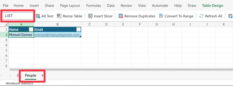
I want to highlight the name of the table “LIST” and the name of the sheet “People”. Sorry for the lack of imagination, but let’s focus on the content here :).
Accessing the Excel Scripts Editor
Open your Excel file either online or in your computer Excel Online and navigate to the "Automate" tab in the ribbon.
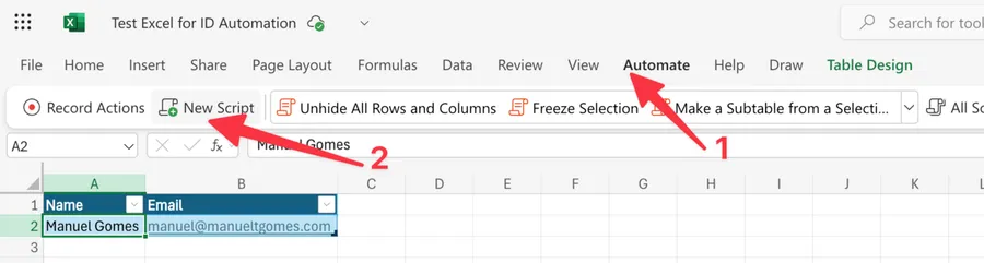
Click on "New Script" to open the Code Editor. You’ll see this.

Click “Write a script”.
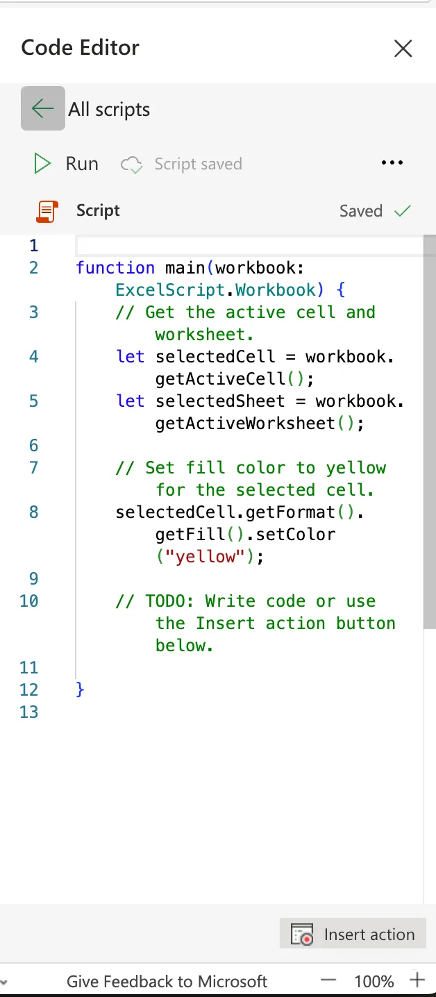
You can remove the code that is there since we’ll write our own.
Before we continue, we will need an Excel ID column, so please add it now if you haven’t already done so. We’ll use “ID” but you can use any name you like.

Notice that I’ve added it to the middle to demonstrate that the column's position doesn’t matter.
Creating the Script
Copy the following code into the script editor:
function main(workbook: ExcelScript.Workbook)
{
    let sheet = workbook.getWorksheet("People"); // This is the sheet's name
    let table = sheet.getTable("LIST"); // This is the name of the table

    let headers = table.getHeaderRowRange().getValues()[0];
    let idColumnIndex = headers.indexOf("ID"); // One column we added
    let nameColumnIndex = headers.indexOf("Name"); // This column will indicate if the row is filled or not

    if (idColumnIndex === -1 || nameColumnIndex === -1) {
        throw new Error("Required columns (ID, Name) not found.");
    }

    let dataRange = table.getRangeBetweenHeaderAndTotal().getValues();
    let updated = false;

    for (let i = 0; i < dataRange.length; i++) {
        let name = dataRange[i][nameColumnIndex];

        if (!name) {
            continue; // Skip empty rows
        }

        if (!dataRange[i][idColumnIndex]) {
            dataRange[i][idColumnIndex] = generateUUID();
            updated = true;
        }

    }

    if (updated) {
        table.getRangeBetweenHeaderAndTotal().setValues(dataRange);
    }
}

function generateUUID(): string {
    return 'xxxxxxxx-xxxx-4xxx-yxxx-xxxxxxxxxxxx'.replace(/[xy]/g, function(c) {
        let r = Math.random() * 16 | 0,
            v = c === 'x' ? r : (r & 0x3 | 0x8);
        return v.toString(16);
    });
}
Click “Save Script”. This will save the script with the name “Script”.
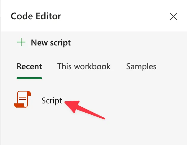
You can customize it to show something more explicit because you can have multiple scripts in the same Excel File. To do that, click the back button with “All scripts,” and you’ll see this.

Click the 3 dots and pick “Rename”. Pick the name you would like and the save it again.
Customizing for Your Excel Structure
Before saving, you'll need to modify the script to match your specific Excel file:
- Change
"People"to your actual worksheet name - Change
"LIST"to your actual table name - Adjust the column names (
"ID","Name") to match your table headers - Optionally add or remove ID columns based on your requirements
Please don’t forget to do this; otherwise, you’ll get some strange errors, or your ID columns won’t be generated.
Saving and Testing
You can run it directly in Excel or in Power Automate. Notice that the IDS will only be generated when the script runs, so having a scheduled Flow that runs it would probably be a better approach, but it’s up to you.
In Excel, run the script using the "Run" button to test it on your data. You’ll see the value added to your file.

To run it in Power Automate you can use the “Run Script” action.
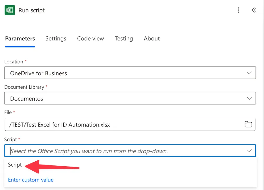
Your script will appear in the dropdown. If you keep the default name, it will be difficult to understand what the script does, so please rename it to something better.
Explaining the script
I’m not an Excel expert, so it’s possible that someone will show me a better script, but since this is also a learning opportunity for me, here’s how the script is built.
Main Function
function main(workbook: ExcelScript.Workbook) {
This is the entry point that Excel Scripts automatically calls when the script runs. It receives the current workbook as a parameter.
Identifying the Target Table and Required Columns
let sheet = workbook.getWorksheet("People");
let table = sheet.getTable("LIST");

let headers = table.getHeaderRowRange().getValues()[0];
let idColumnIndex = headers.indexOf("ID");
let nameColumnIndex = headers.indexOf("Name");
This section:
- Gets a reference to your specific worksheet and table
- Retrieves all column headers from the table
- Locates the exact positions of the ID column and the Name column (which serves as our data indicator)
With this, we can refer to the columns in future actions.
Validation and Error Handling
if (idColumnIndex === -1 || nameColumnIndex === -1) {
    throw new Error("Required columns (ID, Name) not found.");
}
This check ensures that all required columns exist. If any is missing, the script stops with an error message rather than proceeding with incomplete information.
Processing Data Rows
let dataRange = table.getRangeBetweenHeaderAndTotal().getValues();
let updated = false;

for (let i = 0; i < dataRange.length; i++) {
    let name = dataRange[i][nameColumnIndex];

    if (!name) {
        continue; // Skip empty rows
    }
This critical section:
- Get all the data from the table
- Initializes a tracking variable to know if any changes were made
- Loops through each row
- Check if the row has a value in the Name column
- Skips empty rows, ensuring we don't waste GUIDs on unused rows
The skipping part is essential because we don’t want to add data to columns that don’t have data. This will make the script run faster, and we know that if we have an ID, the row has data. I’ve explained it before, but in case you missed it, we check by looking at one column to see if it has data, and then we know that the row has data. Think of this as a column that if it doesn’t have data, then even if the others have it, it’s useless. You can check more columns by replicating that code for the other columns and checking them all simultaneously.
Adding more ID columns if needed.
This is an edge case, but I wanted to show you how to use it. It’s easy, but we must change a few things in the script. Here’s the script, and I’ll show you the changes after.
In this example we’ll add the “DOCUMENT_ID” and “PROFILE_ID”.
function main(workbook: ExcelScript.Workbook) {
    let sheet = workbook.getWorksheet("People"); // This is the sheet's name
    let table = sheet.getTable("LIST"); // This is the name of the table

    let headers = table.getHeaderRowRange().getValues()[0];
    let idColumnIndex = headers.indexOf("ID"); // Primary ID column
    let documentIdColumnIndex = headers.indexOf("DOCUMENT_ID"); // Secondary ID column
    let profileIdColumnIndex = headers.indexOf("PROFILE_ID"); // Third ID column
    let nameColumnIndex = headers.indexOf("Name"); // This column will indicate if the row is filled or not

    if (idColumnIndex === -1 || documentIdColumnIndex === -1 ||
        profileIdColumnIndex === -1 || nameColumnIndex === -1) {
        throw new Error("Required columns (ID, DOCUMENT_ID, PROFILE_ID, Name) not found.");
    }

    let dataRange = table.getRangeBetweenHeaderAndTotal().getValues();
    let updated = false;

    for (let i = 0; i < dataRange.length; i++) {
        let name = dataRange[i][nameColumnIndex];

        if (!name) {
            continue; // Skip empty rows
        }

        // Check and update each ID column as needed
        if (!dataRange[i][idColumnIndex]) {
            dataRange[i][idColumnIndex] = generateUUID();
            updated = true;
        }

        if (!dataRange[i][documentIdColumnIndex]) {
            dataRange[i][documentIdColumnIndex] = generateUUID();
            updated = true;
        }

        if (!dataRange[i][profileIdColumnIndex]) {
            dataRange[i][profileIdColumnIndex] = generateUUID();
            updated = true;
        }
    }

    if (updated) {
        table.getRangeBetweenHeaderAndTotal().setValues(dataRange);
    }
}
So, in this case, we’ll need to do a few things. First, we will have three columns to add data instead of one:
let idColumnIndex = headers.indexOf("ID");
let documentIdColumnIndex = headers.indexOf("DOCUMENT_ID");
let profileIdColumnIndex = headers.indexOf("PROFILE_ID");
Then we need to check if those columns exist or not
if (idColumnIndex === -1 || documentIdColumnIndex === -1 ||
    profileIdColumnIndex === -1 || nameColumnIndex === -1) {
    throw new Error("Required columns (ID, DOCUMENT_ID, PROFILE_ID, Name) not found.");
}
Then, for each row with data, we check and update all three ID columns:
if (!dataRange[i][idColumnIndex]) {
    dataRange[i][idColumnIndex] = generateUUID();
    updated = true;
}

if (!dataRange[i][documentIdColumnIndex]) {
    dataRange[i][documentIdColumnIndex] = generateUUID();
    updated = true;
}

if (!dataRange[i][profileIdColumnIndex]) {
    dataRange[i][profileIdColumnIndex] = generateUUID();
    updated = true;
}
Notice that we check each column individually so that if only one has data missing, we’ll only add it to that column.
Final Thoughts
I know it doesn't look easy, but if you follow the steps, I'm sure you'll be able to do it. One recommendation that I have is to have a template with this already configured. You can pick it up, copy it, and create your files with the scripts.
I wanted to define the whole solution carefully because I'm sure you'll see multiple solutions online for this, and they will work. However, I'm sure this one will work and provide many advantages, or at least save you from headaches.
Please let me know if you have feedback on the Excel scripts or anything else. As I said, I'm not a huge expert, so any improvement and learning opportunity is welcome.


No comments yet
Be the first to share your thoughts on this article!