
Picture a class gradebook that keeps filling up. One column holds the student, another holds the subject, another holds the score, and you want the average score for a single subject without dragging a filter across the sheet every time a new row lands. You could keep re-selecting cells by hand, or you could write one formula that asks the question once and answers it forever.
That's what the "Averageif" function does. It averages the numbers in a range, but only for the cells that meet the condition you set. If you've used the "Sum" function or the "Count" function in Excel to work across a whole column, think of the "Averageif" function as a plain average with a filter bolted on, so you average only the rows that matter.
Where to find it?
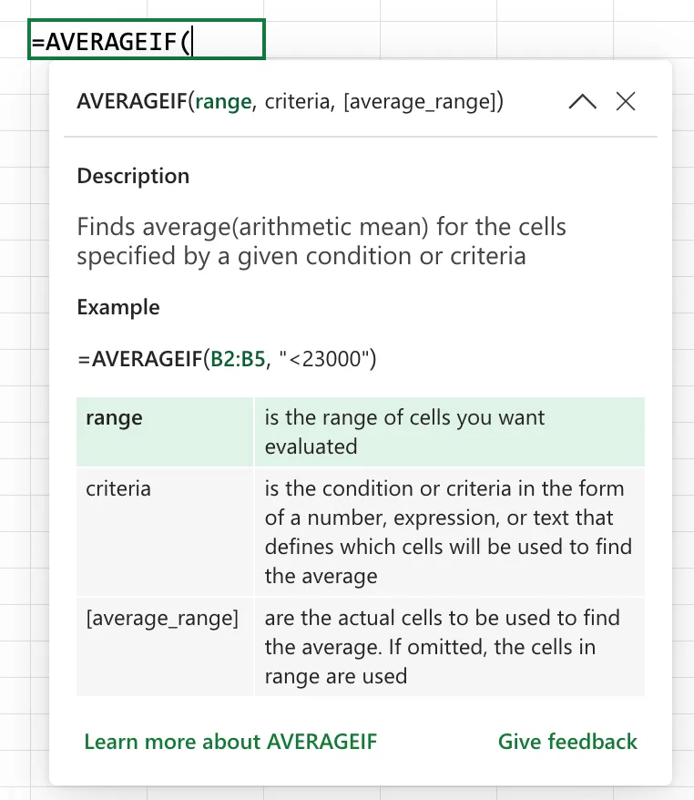
You type the "Averageif" function straight into a cell. Start with an equals sign, type AVERAGEIF, and Excel's formula AutoComplete shows the signature as you fill in each argument. If you prefer a guided experience, you can reach it through the Formulas tab and the "Insert Function" dialog, where it sits under the Statistical category. It works the same way in Excel for Windows, Excel for Mac, and Excel for the web, and it's been available since Excel 2007, so you don't need a Microsoft 365 subscription to use it.
The "Average" function averages everything you give it with no filtering. The "Averageif" function averages only the cells that meet one condition. If you find yourself deleting rows or building a helper column just to average part of your data, the "Averageif" function is almost always the tool you actually wanted.
Usage
You give the "Averageif" function a range to test, the criteria each cell must meet, and (optionally) a separate range whose matching values get averaged. When you leave the third argument out, Excel averages the same range it tested.
=AVERAGEIF(range, criteria, [average_range])
| Parameter | Required | Type | Description |
|---|---|---|---|
| range | Yes | Range | The cells checked against the criteria |
| criteria | Yes | Value or expression | The condition that decides which cells count |
| average_range | No | Range | The cells actually averaged. If omitted, range is averaged instead |
Averaging the same range you test
Let's start with the simplest form. You skip average_range and Excel averages the very cells it checks. This averages every value greater than 10.
Data in A1:A5
5, 12, 8, 20, 30

=AVERAGEIF(A1:A5, ">10")

will return

20.6666...
Only 12, 20, and 30 pass the test, so the result is their average.
Averaging a different range
More often, you test one column and average another. Here you match on the region in column A and average the amounts in column B.
Column A (Region)   Column B (Amount)
North               100
South               200
North               150

=AVERAGEIF(A2:A4, "North", B2:B4)

will return

125
Only the two North rows are averaged, so you get the mean of 100 and 150.
Comparison operators and cell references
Criteria aren't limited to exact matches. Wrap an operator and a value in quotation marks to compare, and join an operator to a cell reference with the & symbol when the threshold lives in another cell.
=AVERAGEIF(B2:B100, ">500")

=AVERAGEIF(B2:B100, ">"&E1)
Wildcards for partial text
Text criteria accept ? to match any single character and * to match any run of characters. This averages the amounts for every region whose name starts with "Nor".
=AVERAGEIF(A2:A100, "Nor*", B2:B100)
The values that finally get averaged follow the usual rules. Numbers count, blank cells in average_range are skipped rather than treated as zero, and cells holding TRUE or FALSE are ignored. That skipping of blanks helps, because it means empty rows don't quietly drag your average down toward zero.
The function family
The "Averageif" function sits in a small group of conditional aggregates that we constantly mix up, so let's put them side by side. Only some of these have a dedicated article yet, so keep this table handy while you pick the right one.
| Function | What it does |
|---|---|
| Average | Averages everything you give it, with no conditions |
| Averageif | Averages the values that meet one condition |
| Averageifs | Averages the values that meet several conditions at once |
| Sumif | Adds the values that meet one condition |
| Countif | Counts the cells that meet one condition |
If you need more than one condition, reach for the "Averageifs" function instead. Its argument order is different, so it isn't a drop-in replacement, but it's the natural next step once a single filter isn't enough.
Real-world examples
Let's look at three situations where this comes up a lot.
A subject average on a busy gradebook
Maria keeps a sheet where every row is one test result, with the subject in column A and the score in column C. She wants a tile that always shows the current average for Mathematics, even as new results arrive.
=AVERAGEIF(A2:A500, "Mathematics", C2:C500)
The formula re-evaluates whenever a new row lands, so the tile stays correct without any manual work.
An average that ignores the zeros
João tracks daily sales, but days when the shop was closed show up as 0 and pull the true average down. Averaging only the days above zero gives a fairer picture of a normal trading day.
=AVERAGEIF(B2:B100, ">0")
A threshold that lives in its own cell
When the cut-off is likely to change, put it in a cell and reference it. Here E1 holds the minimum amount, and the formula averages everything at or above it.
=AVERAGEIF(B2:B100, ">="&E1)
Changing E1 updates the result instantly, and anyone opening the workbook can see the threshold without reading the formula.
Non-intuitive behaviors
An empty criteria cell means zero
When your criteria points at another cell, as in ">="&E1, and that cell happens to be empty, Excel reads the empty cell as 0. The formula doesn't error. It quietly widens the filter and averages everything at or above zero instead of the threshold you meant. Give the threshold cell a default value, or guard the formula, if it can ever be left blank.
average_range is resized to match range
The third argument doesn't have to be the same size as the first. Excel only reads its top-left cell and then rebuilds a block the same shape as range from that corner. So =AVERAGEIF(A2:A10, "North", B2:B5) doesn't average just B2:B5. Excel silently stretches it to B2:B10 to line up with the ten rows in range. The result can look correct at a glance while quietly averaging cells you never pointed at.
Because Excel reshapes average_range from its top-left cell, a mismatched range doesn't raise an error. It just averages a different block than the one you typed. Always give average_range the same rows as range so the formula does what it reads like it does.
Blank matching cells produce a divide-by-zero
If cells do match your criteria but every one of them is empty in average_range, there's nothing to average, so the "Averageif" function returns a #DIV/0! error. This is different from having no matches at all, yet it surfaces the same error, which can make it tricky to diagnose.
Limitations
It handles exactly one condition
The "Averageif" function tests a single criterion. There's no way to say "Mathematics AND above 50" inside one call. When you need several conditions combined, move to the "Averageifs" function, which takes one or more criteria pairs and combines them with AND logic.
Text, logicals, and blanks are left out of the average
Only numbers are averaged. Cells in average_range that hold text or the logical values TRUE and FALSE are ignored, and blank cells are skipped rather than counted as zero. That's usually what you want, but it means a column you thought held 100 numbers might average only the 90 that are truly numeric.
It returns #DIV/0! when nothing qualifies
If no cell meets the criteria, or the range is blank or contains only text, there's nothing to divide, so the formula returns #DIV/0!. Unlike the "Sum" function, which happily returns 0 for an empty selection, an average of nothing is undefined, and Excel says so with an error rather than a number.
Numbers stored as text are invisible to it
A value like "150" that is stored as text isn't a number, so the "Averageif" function neither tests it as one nor includes it in the average. A column imported from another system is the usual source of this, and it can make a formula return far fewer values than you expected.
Localization
The separator between arguments changes with your regional and list separator settings. With some settings it's a comma, and with others, such as Portugal, it's a semicolon. The decimal separator flips too, so a threshold reads ">1000,5" rather than ">1000.5" on those systems.
// Comma-based regional settings
=AVERAGEIF(A2:A100, "North", B2:B100)

// Semicolon-based regional settings (for example, Portugal)
=AVERAGEIF(A2:A100; "North"; B2:B100)
Troubleshooting Common Errors
These are the ones we run into most often, and each has a quick way out.
The formula returns #DIV/0!
Cause: No cell met the criteria, or the cells that did match were all empty, so there was nothing to average. A criterion written slightly wrong (a typo, a trailing space, or a date compared as text) filters everything out and lands you here.
Solution: Test the criterion on its own first, then wrap the formula in the "Iferror" function so an empty result shows a friendly value instead of a red error on your dashboard.
=IFERROR(AVERAGEIF(A2:A100, "North", B2:B100), 0)
The average is lower than expected
Cause: Genuine zeros are being counted when you meant to skip them. Days with no trading, rows that were filled in with a literal 0, and imported placeholders all pull the average down toward zero.
Solution: Tighten the criterion so those zeros fall out. Averaging only values above zero is the common fix.
=AVERAGEIF(B2:B100, ">0")
The result ignores rows you can clearly see
Cause: The numbers you expected to average are stored as text, so the "Averageif" function doesn't recognize them as numbers. Text values often arrive from a copy-paste or an import and sit left-aligned in the cell.
Solution: Convert the column back to real numbers. Selecting it and using the "Value" function or the Text to Columns tool restores them, after which the formula picks them up.
The average_range averages the wrong cells
Cause: average_range is a different size from range, so Excel reshaped it from its top-left cell and averaged a block you didn't intend.
Solution: Give average_range exactly the same rows as range. Aligning A2:A100 with B2:B100 (not B2:B50) makes the formula average what it reads like it should.
Recommendations
Here are some things to keep in mind.
Line up your two ranges
Because Excel quietly reshapes average_range to match range, decide on your row span once and use it for both arguments. Named ranges make this almost automatic and keep the formula readable as the sheet grows.
=AVERAGEIF(Region, "North", Amount)
Keep thresholds in cells, not inside the formula
When a condition is a moving target, such as a minimum score or a cut-off amount, put it in its own cell and reference it with &. You change one cell instead of editing the formula, and the intent stays obvious to whoever opens the workbook next.
=AVERAGEIF(B2:B100, ">="&E1)
Decide what zero and blank should mean
An average is only as honest as the rows feeding it. Before trusting the number, decide whether empty cells and literal zeros belong in it, then shape your criterion to match that decision. A quick ">0" often turns a misleading average into a truthful one.
Always deal with errors
A missing match returns #DIV/0!, and that error spreads into any cell that references it. Wrap the formula in the "Iferror" function or clean the source data so one empty result doesn't break the report that depends on it.
=IFERROR(AVERAGEIF(A2:A100, "North", B2:B100), 0)
Final Thoughts
The "Averageif" function turns a filter-and-average chore into a single formula that keeps working as your data grows. Remember that it handles one condition, that it skips text and blanks but returns #DIV/0! when nothing qualifies, and that Excel reshapes average_range to match range whether you meant it to or not. Keep those three in mind and it becomes one of the most dependable tools in your workbook.
Sources
Back to the Excel Function Reference
Photo by Jesús Vidal on Unsplash



No comments yet
Be the first to share your thoughts on this article!